Book summary: Predictably Irrational

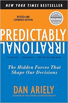
A future work colleague recently recommended a book to me that might be useful as a consultant working with data. It's called Predictably Irrational, by Dan Ariely, and it contains a catalogue and commentary on some of the cognitive biases that cause humans to make irrational decisions, particularly in economic settings. He describes experiments (both virtual and real) that demonstrate the effects, argues for their pervasiveness in our lives, and proposes ways to mitigate them.

I wanted to put up this post as a summary of the book and a record of some of my reactions to it, which will hopefully force me to read actively rather than skimming. Hopefully you'll find it useful too.

Summaries of chapters are on the left in black,

my reactions are on the right in purple.

Introduction

Economics is based on a model that says humans make rational decisions according to their preferences, and with complete information. In contrast, behavioral economics considers that people sometimes make irrational decisions. These decisions are not random, however, but can be tested experimentally and predicted. Some of these errors may be mitigated by learning about the forces that shape our irrational choices.

I was just writing about how cognitive bias takes a back seat in data science, but it's driving the car in this book. Having read Dan Kahneman's Thinking, Fast and Slow and spent some time on lesswrong.com, I'm familiar with the concept. It sounds like this book is principally concerned with cognitive bias as it applies to economic decisions, which I assume will be useful in my job. I don't know what Ariely's motivation is yet - is he going to teach us how to use behavioral economics to sell more hamburgers, or to make sure we buy the best hamburger? 

1. The Truth about Relativity:  Why Everything is Relative -- Even When It Shouldn't Be

It's hard to assess the value of something unless it's compared to other similar things. Given three options (A, B, C) with B and C being similar but B superior to C, people will tend to choose option B regardless of the quality of A. This is called the decoy effect. Ariely suggests that it's partly responsible for the creep of materialism, in that when we buy a car we tend to compare it to slightly better cars. He also suggests that to limit the decoy effect's effect on us, we can try to limit the options we have access to. Experiments are presented that show that the effect is real and strong.

I hadn't really thought about how pervasive this effect is in our lives. Ariely points out that it's responsible for the "wingman effect," where you can bring a less attractive friend to a bar when you're looking for a date. You not only look better compared to your friend, but to the rest of the bar as well. It's also used extensively in advertising to make us "creep" up to more expensive items or packages. 

Ariely's writing is very conversational and a bit hyperbolic. The analysis is qualitative, and it's not exactly clear how strong this effect is, and whether the results are statistically significant. I'm interested in how the decoy effect competes or cooperates with updating preferences based on prior information. We don't assign value to a set of speakers without hearing similar speakers in part because we haven't heard any of the speakers yet.

I'm somewhat surprised by the suggestion that we intentionally and artificially limit our access to options in order to curb this effect. This is not the usual approach to cognitive bias, but it's consistent with the view that ignorance is bliss.

2. The Fallacy of Supply and Demand: Why the Price of Pearls -- and Everything Else -- Is Up in the Air

The law of supply and demand is supposed to set the price of goods and services, but this is based on a rational economic model. In reality, the price of things is pretty arbitrary. Ariely introduces the concept of arbitrary coherence, where prices and behaviors may be based on previous prices or behaviors, but the original ones were set arbitrarily. He uses the well-known bias of anchoring, in which our beliefs about numerical quantities are influenced by numbers we've seen or heard recently, even if they have no logical connection. He talks about some experiments he's done that show that not only does anchoring affect the price we're willing to pay for something, but it can even make the difference between being willing to pay for something or demanding to be paid for it, if the thing in question has ambiguous value.

He also shows that the influence of anchors is long-lived: you can't replace them with new anchors easily. Some theories as to why we are willing to pay so much for Starbucks coffee are put forward (we don't compare to similar products because of the difference in atmosphere).

Ariely also talks about self herding, in which we think about how often we've done something before, and take that as independent evidence that that thing is good to do. This shores up the theory that our habits may be quite arbitrary at their roots. His advice is to become aware of these vulnerabilities and question our habits. Consider the rewards and costs of each decision. Mathematically speaking, this theory suggests that supply and demand are not independent, but coupled.

We tend to rationalize our choices after the fact, and Ariely argues that this might not be a bad thing as long as it makes us happy.

Arbitrary coherence is an interesting idea. It reminds me of filamentation in nonlinear optics, or actually just anything in nonlinear optics. Or just anything nonlinear with a random seed. It also a pretty bold claim, and I've never heard anyone else make it. Granted, I don't run in sociological circles. I'll have to run it by some friends. Self-herding as a mechanism is sexy.

This chapter leaves me wanting to see some equations. What happens formally when you assume various kinds of coupling terms between supply and demand? Surely this is solved. I assume it results in prices that are either saturating exponentials, oscillatory functions, or hyperbolic trig functions. This seems like a simple opportunity to extend conventional economics into the field of behavioral economics.

Finally, I feel strongly that rationalization is bad. If you have arbitrary preferences for one car over another one, they can be taken into account formally using decision theory. Even with the craziest preferences in the world, you can still make consistent decisions as long as you don't violate a few axioms. As soon as you allow ad hoc rationalization, decision theory goes out the window. That's a sacrifice I'm not willing to make.

3. The Cost of Zero Cost: Why We Often Pay Too Much When We Pay Nothing

People respond to a cost of $0.00 differently than to other similar costs. For example, consider the following two situations.

People make decisions about these choices as if the relative value of A over B were much greater in Choice 1 than Choice 2, even though the difference in cost is identical, and $0.01 is certainly below the wealth-depletion regime. He gives an example of Amazon, where the inclusion of free shipping for orders above a threshold entices people to spend more than the cost of shipping, and points out that this does not work if they reduce the cost of shipping to a few cents.

He also mentions a thought experiment where you are given a choice between two gift certificates (again, for Amazon). The first is a free $10 gift card, and the second is a $20 gift card that requires you to first pay $7. He speculates that people would be more likely to choose the first.

Seems reasonable. I take issue with the Amazon example though. One one hand, suppose we replace "Amazon" with "turpentine factory." I don't value turpentine, so the decision to take the free option is quite rational. Now suppose we replace "Amazon" with "cold, hard cash." Everyone would obviously choose the second option because everyone values cash as much as cash. So the question seems to depend on how much we value the commodity. I don't see why that's irrational. 

4. The Cost of Social Norms: Why We are Happy to Do Things, But Not When We are Paid to Do Them.

There are market norms, and there are social norms, and it seems that people act as if there is a sharp division between the two. For example, We don't offer payment for a family Thanksgiving dinner, but we might bring an expensive bottle of wine. Essentially, if we apply social norms to situations we tend to undervalue our own time and effort. 

Companies try to sell us things by trying to forge a connection to us. Open source software is another example, where very skilled people spend a lot of their time to work, but would not do so for a small amount of money. Ariely hypothesizes that this effect is responsible for police being willing to risk their lives for relatively small amounts of money. 

Now I feel like we're getting somewhere. This is a familiar concept of course, but this chapter puts it in concrete terms. It reminds me of the subscription program on Twitch.tv, where I subscribe to people for essentially no personal benefit. It puts a name to the awkwardness I feel offering money to friends when they babysit for me. 

It also calls to mind the office culture in my soon-to-be office. They have a family-like atmosphere,  unlimited paid time off, and even award a bonus for taking seven consecutive days off during the year. This may be effective at generating more committed workers. 

I wonder what kind of norms are at play in academic research science. It is certainly true that the amount of money I made was far below what I could have made in the private sector. I also reviewed papers for free even though I paid publication fees when I had papers accepted at journals. Was I motivated by social norms like the quest for scientific truth, the solidarity between academic scientists in a similar situation? Or was I motivated more by the eventual promise of tenure, which is a market-like reward?

5. The Power of a Free Cookie: How Free Can Make Us Less Selfish.

If something is free instead of cheap, we tend to regulate it with social norms instead of supply and demand. So if you offer a tray of free cookies to a group of people sequentially, they will tend to take a small number of cookies. But if you sell those same cookies for $0.05 each to those same people, people tend to buy many of them, even though five cents is basically free.

Ariely suggests that this phenomenon will keep programs like cap-and-trade from working. By putting a price on pollution instead of making it free, companies may feel free to pollute more, since they've paid for it, whereas if it were free they might be bound by social norms.

This seems reasonable, and I can think of anecdotal evidence to support it. Ariely's experiments also show it to be true. I have reservations about his statements on cap-and-trade, since I think the total amount of credits is kept constant. The companies couldn't pollute more in total than before. I also don't think companies are bound strongly by social norms in the first place, but that's speculation on my part.

Frankly, I feel pretty bad when I buy all of something cheap at a grocery store, similar to how people apparently treat free things. Not sure how sharp this division is.

6. The Influence of Arousal: Why Hot is Much Hotter than We Realize.

Ariely describes some fairly interesting experiments that demonstrate two things. (1) We make different decisions when sexually aroused, and (2) we can't accurately predict how different those decisions will be ahead of time. The first of these is pretty obvious, and the second is less obvious and a little worrying.

Specifically, test subjects were more likely to agree to propositions like "I would not use a condom if I thought my partner would chance his/her mind while I went to get it" while aroused than while not aroused. In light of this, Ariely suggests that asking teens to make good decisions while heated up is basically useless. If we want to prevent pregnancy and STD transmission in teens, we either need to keep them from being aroused, or we need to make things like condoms so universally available that teens never really have to think about whether to use them or not.

In this chapter Ariely makes explicit what he's only implied before: in his model of human thought, we are like Dr Jekyll and Mr Hyde. The latter makes decisions that the former would not agree with or necessarily predict correctly. He also brings up id, ego, and superego more than once, and paraphrases Sigmund Freud. He goes so far as to say that "We may, in fact, be an agglomeration of multiple selves." Not being a psychologist, I'm not sure what to make of this model. It was my understanding that Freud's theories were no longer thought to be an accurate description of psychological phenomena, but maybe I'm wrong. In any case, it seems that there should at least be a continuous transition between Dr. Jekyll and Mr. Hyde.

7. The Problem of Procrastination and Self-control: Why We Can't Make Ourselves Do What We Want to Do.

People don't save as much money as they used to, and also not as much as they say they want to. In fact, the average US family has thousands of dollars of credit card debt. People also procrastinate, and are often looking for ways to avoid it. In this chapter, Ariely tells a success story of Ford Motor Company, who managed to get people to follow their maintenance schedule by simplifying it at the cost of part efficiency (i.e. some parts were inspected before it was strictly necessary). He suggests that a similar idea might be applied to medicine, where people tend to fail to get routine checkups done.

He also pitches an idea for a credit card where consumers could decide ahead of time how much money they wanted to spend on certain categories of goods, and what penalties they would face if they attempted to exceed these limits.

Just yesterday I was doing some Pomodoros, which is a way of setting an artificial deadline. Ariely's advice for overcoming procrastination also includes rewarding yourself for doing things you don't wan to do, which is pretty standard advice.

A bit off subject, I'm wondering how much confirmation bias is coming into play while I'm reading this book. Am I too willing to accept that these effects are real? After all, the experimental data are presented anecdotally, with no statistical significances quoted. The person designing them could in principle have fallen victim to any number of well known biases in scientific studies. For the moment, my own recognition of these effects in my life is suspending my disbelief. It's making me very curious to what degree we can quantify these effects.

8: The High Price of Ownership: Why We Overvalue What We Have.

People tend to assign higher value to what they have, and lower value to what other people have. The main experiment presented in this chapter involved interviewing students who had won Duke basketball tickets in a lottery. Owners quoted an average selling price of $\$2400$, and non-owners quoted an average buying price of $175 - a huge difference. Both owners and sellers were more concerned with what they had to lose in the sale than what they had to gain. Ariely speculates that part of this effect comes from the transferrence of our emotional attachment to the buyer. Also, buyers are ignorant of the emotional history that the seller has to a house or a car.

This effect is important on auction sites like Ebay, where "partial ownership"  - the feeling of ownership generated by leading a bidding war for some time - might explain overbidding in the last few minutes of the auction. It also may apply to politics, religion, or other ideologies. We value the ones we hold and undervalue those of others.

How does this compare to "the grass is always greener on the other side of the fence," - where we tend to undervalue what we have and overvalue what others have? Could we set up similar experiments to demonstrate exactly the opposite effect? Could we set up an experiment that quantifies the relationship between these two effects?

9. Keeping Doors Open: Why Options Distract Us From Our Main Objective.

People tend to avoid committing to a single option when many are available, and will sacrifice expected value in order to keep these options available. In experiments, subjects were given a screen with three doors to open. Clicking inside each door gave a randomized payout, and subjects had a limited number of clicks to spend. They turned out to be pretty good at adapting their strategy to maximize expected value. Then a new condition was added, where after 8 consecutive clicks elsewhere a door would be locked permanently. Subjects preferred to jump around keeping doors open, even when the expected value for each door was advertised.

Ariely advises us to focus down on a smaller number of opportunities, and stop investing in things that are getting us nowhere, explicitly citing a woman he knew trying to choose between two boyfriends. He goes so far as to suggest that we "stop sending holiday cards to people who have moved on to other lives and friends." He also models the US Congress as a person reluctant to choose one option among many, which leads to gridlock.

I have a few issues with this chapter. The results of the door experiment are completely nuts, first of all. I can tell you that neither I or my poker buddies would think twice about letting a low-EV door close permanently. In fact, I wonder how robust these effects are against training. I know for example that anchoring is almost impossible to avoid even by experts at cognitive bias studies. Maybe this "commitment bias" is less robust.

Second, while I understand that failing to commit to a serious relationship can have bad consequences, I'm pretty sure that sending holiday cards has basically zero cost. I don't know why cutting off old friends is going to improve my life unless I'm spending so much time writing Christmas cards that I don't have time to hang out with my other friends.

Third, congress is in deadlock not because it's a single entity that fails to commit to a course of action, but because it's made of at least two entities completely committed to conflicting courses of action. I don't see why this bias applies.

10. The Effect of Expectations: Why the Mind Gets What it Expects.

The basic message of this chapter is that our experience depends on what we expect from it. Expensive wine tastes better, even if it's identical to cheap wine. World-famous classical musicians play unnoticed in subways. It's also be responsible for brand loyalty to some extent. MRI images taken from people drinking Coke and Pepsi show that the area of the brain associated with higher functions is preferentially active for Coke, meaning that it's not simply a taste experience, but also a memory experience. Ariely makes a few suggestions to help us make less biased decisions, which involve blinding ourselves to labels.

The mere fact that prior information influences our beliefs in a subjective way is not interesting - it's a fundamental tenet of probability theory. The interesting thing here is that it changes our perception in a way that depends on the time that we learn the information. For example, in a taste test, our reported experience depends strongly on whether we learn the labels before or after tasting, even if reports are made after everything.

Ariely says something interesting in this chapter. Regarding manipulating people's expectations intentionally, he says "I am not endorsing the morality of such actions, just point to the expected outcomes." So he explicitly takes an agnostic position on the ethics of learning about or using cognitive bias effects.

11. The Power of Price: Why a 50 Cent Aspirin Can Do What a Penny Aspirin Cannot.

This chapter covers the placebo effect. In experiments, pills labeled as more expensive work better. In another experiment, an inert drink was offered as a physical or mental boosting agent and had the advertised effect. Ariely suggests that it is ethical to exploit the placebo effect by intentionally prescribing them. He also comments on the ethics of experiments which test whether a treatment functions through the placebo effect.

This seems to be a special case of chapter 10's discussion of expectations. I'm interested in the ethics discussion. By now it's clear that Ariely is in favor of exploiting cognitive bias to put ourselves in positive situations, as opposed to attempting to eliminate it.

12. The Cycle of Distrust: Why We Don't Believe What Marketeers Tell Us.

People are always looking for a catch. In an experiment literally giving away free money to passersby on a college campus, only 20% of people took a $50 bill. Ariely also discusses the Tragedy of the Commons, which is a game theory scenario in which cooperation is optimal but unstable. Defection is preferred over the short term, but causes everyone to lose in the long term.

Examples are given of companies who were able to recover from PR disasters by sustained transparency efforts. Ariely says that companies can get away with lying to some small extent, but then they lose people's trust. Once it's gone it's very hard to regain.

In another experiment, people were very willing to accept obviously true statements like "the sun is yellow" if they came from unnamed sources, but if attributed to entities like Proctor & Gamble or The Democratic Party, they became suspicious (specifically, they started wondering about orange or red colors in the sun). This showed that they were looking for excuses not to believe these entities.

This chapter drives home that trust and distrust don't just cancel out when it comes to people and companies (also probably people and people). Maybe obvious in retrospect, but worth noting. Not sure I have anything more to say about that.

13. The Context of Our Character, Part 1: Why We Are Dishonest, and What We Can Do About It.

This chapter is about dishonesty, and how we think about dishonesty involving cash as different from other dishonesty, even when it has greater equivalent cost.

White-collar crimes cause much financial damage than, say, petty theft. We put lots of resources into dealing with the latter, and very little into dealing with the former. Ariely conducted an experiment at Harvard, which gave people an opportunity to cheat when reporting test scores, in a setting where better scores earned more money. He found that people cheated to a small degree when given the opportunity, but that varying the risk of being caught didn't have much of an effect. He also exposed test subjects to neutral text as well as the Ten Commandments before the test, finding that the latter group cheated less.

He suggests that requiring various professionals to take oaths of honesty policy would curb cheating, even without enforcement.

Again, Ariely uses Freud and the concept of the superego to explain this phenomenon. He states that criminals do not perform cost/benefit analyses before committing crimes. I don't know whether this is true, but I'm sure I personally would do such an analysis.

14. The Context of Our Character, Part 2: Why Dealing With Cash Makes Us More Honest.

People cheat more when cash is not directly involved, even when the link to cash is explicit. In an experiment similar to above where test takers won tokens immediately redeemable for cash, cheating increased significantly. Ariely points out that the rates of cheating measured in this experiment should be taken as a baseline, having been done on otherwise honest students in controlled conditions, with the implication that real-world cheating should occur at a much higher rate. He also contends that companies are very happy to cheat consumers out of money as long as it's not technically cash. He uses blackout days of frequent flier miles as an example: having to spend more miles to make a purchase is effectively equivalent to having to spend more cash.

The results of this experiment were surprising to me, and this is the kind of thing I don't feel like I have a good intuition for. People fail to make consistent decisions when cash vs. cash equivalents are involved. I assume this has implications not only for security, but also for marketing. I'll have to reflect on this for a while.

15. Beer and Free Lunches: What Is Behavioral Economics, and Where Are The Free Lunches?

Ariely discusses an experiment he ran in which he gave away free beer. Given four choices of beer, groups of people tended to disproportionately choose different beers from each other when asked to order out loud in series. Others ordered in secret and tended to gravitate to some beers more than others. When asked to rate the beers afterward, people rated the beers higher if they were ordered in secret. This implies that people are willing to sacrifice expected value in order to appear to be unique.

By "free lunch," Ariely is referring to win-win situations. He suggests that behavioral economics may be able to find many such lunches.

The beer experiment seems to be in conflict with what we've learned about ownership bias. If I chose some particular beer,  wouldn't I be likely to overvalue it and rate it highly? Even so, maybe the effect causes a constant bias regardless of whether it was a secret or public order. The main lesson of the book, Ariely says, is that we are "pawns in a game whose forces we largely fail to comprehend." Or in other words, if you think you're making rational decisions, you're fooling yourself.

Final Thoughts

I learned about a few new things from this book, so I'm happy I read it. I suspect that some of these ideas will be useful in my new job, but it's hard to know for sure without context. Already I'm seeing certain of these biases in my everyday life, which is a good indicator that I've internalized some of this information.

It's not clear to me how strong these effects are, particularly with respect to each other. I wonder to what extent they can be quantified. Ariely has convinced me that they influence our behavior to some degree, but without a full statistical analysis it's hard for me to know how much confidence to have in each one. The premise of the book is that we can predict irrational behavior, but it's going to make decisions without a quantitative measure, i.e. the probability and magnitude of an irrational decision.

I'm more interested in the way Ariely advocate dealing with cognitive biases. His stance is not that we try to eliminate them, or even adjust our calculations to account for known biases, but instead to embrace them. We should put ourselves in situations where our biases lead to good decisions, which may involve limiting the information we allow ourselves to access. And we should recognize that if we are happy because of a bias, that still counts as being happy. It may not be worth trying to correct a bias when doing so would ultimately make us less happy.

Ariely doesn't say anything about the ethics of using these biases to manipulate others, even though he does indeed suggest that certain manipulations would work. I'm looking forward to discussing this with more of the data science community as I meet them.

New job

I started this blog the day after I decided to begin a career transition, so that would be May 12th of this year. It's been six months and 23 days since then, and I have to say that things have gone just about as smoothly and quickly as they could have gone.

Last Friday, the 4th of December, I signed a work agreement to be a data scientist at a consulting company starting in January. They work with media and technology companies to better market their products. The company has a great culture and some very smart people, and I'm extremely excited to start. I now feel comfortable calling myself a professional data scientist.

The question now is what to do with the blog. It was intended to serve two purposes: build a portfolio, and help other people with a similar transition by talking about my experience. The former goal seems moot now, and I only need a few more posts to talk about the latter. I think the most likely thing is that I'll finish those posts and then start a new blog about data in general.

Specifically, I'm interested in the culture of data science and how it relates to research science. I would like to become a voice in the community, but I'm not sure yet what I have to say. Let's find out.

Digit recognition part 2: a validation pipeline

[Link to part 1]

I've been looking recently at the MNIST data set, which contains thousands of hand-written digits like this:

Example hand-written numerals from the MNIST data set

where we also have a label for each digit $\in \left[0,9\right]$. We would like to use these examples to assign labels to a set of unknown digits.

In part 1 of this series, I looked at the data set and did some preliminary analysis, concluding that:

1. There's not much variance within each digit label, i.e. all 5's look pretty much the same.
2. Most inter-numeral variance occurs near the center of the field, implying that we can probably throw away the pixels near the edge.

Rather than jumping right into optimizing a classifier in part 2, I'd like to build a validation pipeline. Any time we do machine learning, we want to try to quantify how well our regression or classification should perform on future data. To do otherwise is to leave ourselves prone to errors like overfitting. Validation in this case will apply the classifier to a new set of digits, and then compare the predicted labels to the actual labels.

The Methodology

Here is a pretty concise description of the usual validation methodology. Basically, we break the data into three chunks before we start: a training set, validation set, and test set. Every time we train a classifier we use the training set, and then evaluate its performance using on the validation set. We do that iteratively while tuning metaparameters until we're happy with the classifier, and then test it on the test set. Since we use the validation set to tune the classifier, it sort of "contaminates" it with information, which is why we need the pristine test set. It gives us a better indicator of how the classifier will perform with new data.

The pipeline

What do we want our validation suite to look like? It might include:

1. Standard goodness-of-fit scores, like precision, accuracy, or F1 scores.
2. Confusion matrices, which illustrate what numerals are likely to be assigned which incorrect labels (e.g. "6" is likely to be labeled "8")
3. Classifier-specific performance plots to evaluate hyperparameters, like regularization constants. These show the training and test error vs. each hyperparameter.

Example: logistic classification

It will be helpful to have a classifier to train in order to build the validation pipeline, so let's choose a simple one. A logistic classifier is a logistic regression in which we apply a threshold to the probability density function to classify a data point. Besides being simple, it's also not going to work very well. For illustrative purposes, that's perfect. I'd like to look at how the performance changes with the hyperparameters, which won't be possible if the performance is close to perfect.

I'm using IPython Notebook again, and I've uploaded the notebook to GitHub so you can follow along, but I'll also paste in some code in case you just want to copy it (please copy away!).

We're just going to use the logistic regression functionality from SciKit-Learn. First I import the data and split it into three groups. 70% goes to training, and 15% each to validation and test sets.

Partitioning the data into training, validation, and test sets.

Here I implement a logistic regression with a linear kernel from SciKit-learn. To do some basic validation, I'll just choose a regularization parameter (C in this case) and train the classifier.

Then we can create a validation report, which includes precision, recall, and F1 score for each numeral. 

It's a bit easier for me to parse things in visual format, so I also made an image out of the confusion matrix. I set the diagonal elements (which were classified correctly) to zero to increase the contrast.

Whiter squares indicate more misclassifications. We see that the most frequent mistake is that "4" tends to get classified as "9", but we also tend to over-assign the numeral "8" to inputs of "1", "2", and "5". Interestingly, this is not a symmetric matrix, so for example we tend to assign the right label to "8" as an input.

Hyperparameters

If we stick with models that are linear in each pixel value, the only hyperparameter we need to choose for logistic regression is the regularization constant, which controls to what degree we weight the input pixels. The two common regularization choices I'll consider are are $l2$ (ridge regression or Tikhonov regularization), and $l1$ (lasso). The former tends to result in a "smooth" weighting, where we put similar weights on everything, but the total overall weight is small. The latter results in "sparse" weighting, where we eliminate many of the inputs as being noninformative. 

If we regularize too little, we'll find that while we have low fit error on the training set, we have large errors on the validation set, which is called overfitting. If we regularize too much, we'll find that we're ignoring important information from the input, resulting in large errors for th training and validation sets. This is called underfitting, and the error is called bias.

It can be useful to plot the training and validation error as a function of the regularization constants to see where the regularization performs best. And since we have a pretty large data set, I'll take only a small fraction of the training set. This will make the training go faster, and will just give us an idea of the parameters we should use in the classifier. Let's look at l2 regularization first.

In this plot, larger values mean that the classifier is doing a better job, with 1.00 implying perfect classification. On the horizontal axis, larger values mean less regularization. The red squares show that as we weaken the regularization, the classifier does a better job with the training data. But the performance on the validation data improves for a bit, and then slowly degrades. So for very little regularization, we have overfitting. From a probabilistic point of view, the classifier is no longer representative of the ensemble from which we draw the data.

The validation score peaks around $C\approx 10^{-2.5}$, so even though I've trained on a small subset of the data, I would use this value moving forward.

Now let's make the same graph using $l1$ regularzation.

The same trends are present here, but the exact value of the optimum is different - around $C\approx 10^{-5.5}$. As a nice illustration, we can run the classifier with this value and see which pixels it elminates. To do that, we retrieve the coefficients from the classifier, of which we get one per pixel per numeral. Keeping only those pixels whose coefficients are $>0$ for at least one of the numerals generates this map:

So to recap, white pixels are those the classifier decides to keep if we tell it to get rid of the least informative ones. Compare this to our map of the variance of each pixel:

and we see that our hunch was correct. The classifier preferentially kept the high-variance pixels.

Now that we have this pipeline, we should be able to use it for other classifiers. The exact analysis will likely change, but at least we'll have a basis for comparison.

What has surprised me about data science

It's been six months since I decided to become a data scientist, and I want to take a moment to reflect on what's been surprising about the journey. When I started, I had a study plan that involved machine learning and statistics courses, and plenty of programming practice.

Surprising things about the physics -> data science transition:

1. Data scientists love hypothesis testing. Specifically, they are serious about binary hypothesis testing, and they tend to take the classical view of null and alternative hypotheses. In business this is called A/B testing, and it's used to make high-impact decisions at major companies every day. This surprises me because I didn't run into formal hypothesis testing very much in physics (although it's more popular in biology, for example). On the other hand, we expect that anywhere people stand to make or lose money based on decisions, those decisions should probably considered formally. The emphasis on hypothesis testing is symptomatic of rationality, but we have to be careful about defining the hypothesis space. Not everything that seems binary is binary.
2. Cognitive bias takes a back seat. I'm used to thinking about rationality as the study of a trifecta of concepts: decision theory, probability, and cognitive bias. People in DS seem very concerned about the first two, while the third is just kind of kept in mind while we do our analysis. It's a hidden variable that causes the results of A/B tests to come out the way they do, and it plays a role in the way we communicate our results to the decision makers. But there doesn't seem to be much attention paid to the pitfalls of cognitive bias in our own analysis. I also haven't found anyone trying to exploit it to influence decisions, even though many data scientists work in marketing. I wonder if this is a place where I can contribute with a unique skill set.
3. Statistics is hard. I thought I would be able to knock this out really quickly since I'm extremely comfortable with probability, but that has not been the case. Part of the problem is that it's typically taught from a tool-oriented viewpoint. We learn that in situation $A$, with $N$ samples from $M$ ensembles, test $X$ is appropriate. Contrast this with the bottom-up approach of Bayesian probability, where we start with the question of how to define a measure of likelihood, and we write out a complete hypothesis space before any problem. This may be why concepts like confidence intervals and p-values are commonly misunderstood even by expert practitioners. I have struggled to reconcile the tools of statistics with the formal logic of probability theory, but I can at least use the tools appropriately. The rest will come with practice.
4. Machine learning is easy. Or at least, for most problems. ML makes up a large percentage of the data science news and tutorials I see, and there's a lot of emphasis on figuring out when to apply which method (again, a tool-oriented approach). But in basically every real example I've found, you can throw any classifier at the problem and it's pretty much OK. Furthermore, unless you have a huge amount of data or a very large parameter space, you can set up a pipeline in Python that tries different classifiers with different hyperparameters (like regularization parameters) and find the one that performs best. You just have to be careful about setting aside test and validation sets. All this to say that we can often afford a brute-force approach to machine learning.
5. Interviews take a lot of resources. I had assumed that it would be rational for companies to do phone screens for any candidate who was possibly qualified for a position, since it's well known that resumes are not good predictors of success. By asking specific technical and non-technical questions, I assume that a competent hiring manager could separate the wheat from the chaff. Sending a data challenge seems like a similarly good idea. But this ignores the fact that even half-hour phone screens require time and effort that's not being put toward high-priority projects, and that someone has to review the data challenge results, which is a lot like grading a test. Which sucks. So it seems like companies are still sort of stuck choosing interviewees based on resume keywords. Seems like a bad idea, but I don't have a great solution.
6. People are afraid of hiring academics. This is something Kathy Copic mentioned at a panel I attended, and it sounded ridiculous at the time, but I can tell you that it's absolutely true: managers are afraid of hiring "stereotypical" academic researchers, who prefer to work alone on very difficult problems for a long time, and generate theoretically perfect results that are of no use to anyone. They also prefer well-defined problems, are not intellectually agile, and are culturally incompetent. I don't know if this fear is founded - maybe there are horror stories about previous hires who fit this description. But a good academic does none of these things either: she works efficiently on small problems in pursuit of bigger ones, adapts her strategy according to previous successes or failures, and is able to collaborate with others and communicate her results.

That's it for now. Thanks for reading!

Digit recognition part 1: visualization

I'd like to move more toward problem-based posts rather than tool-based posts, and today I'm looking at the famous MNIST (Modified National Institute of Standards and Technology) dataset of handwritten digits. These data are available at Kaggle, for example, where there is a training "competition" to use machine learning to identify new digits based on a training set. I'm going to ignore the test set for now and just work with the training set.

In the first part of this series, I just want to get a feel for the data: visualize it and do some preliminary analysis, as if I were not familiar with the problem at all. I'll be working in an IPython notebook. If you want to follow along, I uploaded it to Github.

The data

The data consist of about 40000 digitized handwritten numerals $\in$ [0, 9]. Each numeral was digitized on a 28x28 pixel grid. These grids have been flattened into rows of 784 pixles and stacked together into a 2D array that looks like this:

Each pixel has an intensity value $\in$ [1, 256]. Here's what the raw data array looks like if we just plot it:

Each row can be reconstructed into a 28x28 array. Here are some examples of random reshaped rows:

The information

Eventually we'll want to train a classifier with these digits, and will want to figure out which features (pixels) are important, and which ones aren't. There are plenty of ways to do that automatically, but it's also straightforward to poke at the data a bit and figure it out ahead of time. First, let's make sure we have the same number of examples for each numeral. The raw data array actually has a prepended "label" column that I didn't mention above, which is just the numeral index, 0-9. We can use this to make a histogram:

where we see that there are about 4000 examples of each numeral.

Next, let's look at what range of intensities we have. Making a histogram of all of the intensities for the entire data set, we see the following:

where it's clear that the data mostly consist of black and white pixels, and not much in between. This gives us a hint that we could binarize the data set without losing much information. It also might mean that there's been some pre-processing done on the data set.

How much does each numeral change throughout the data set? We can get some intuition by grouping examples of each numeral and then plotting their means and variances.

Means of each numeral

Variances of each numeral

These two plots contain more or less the same information - that the variance is concentrated near the edges of each numeral, and there isn't too much variance within each numeral, i.e. there's nothing crazy going on here. Compare this to the average and variance taken over all of the numbers.

We expect variance to correlate well to information, so these images show that most of the information is clustered in a blob near the center, which isn't too surprising. We could probably throw away a bunch of the outer pixels without too much trouble. Let's quantify that.

Suppose we order these pixels by variance (descending) and plot the cumulative variance by pixel. That is, show how adding the next largest variance increases the total variance. That gives us an idea of how many pixels we need to capture most of the variance, which we can expect to be related to information content.

The green line is set at 90% of the total variance, which intersects the cumulative variance at about 290 pixels. So through this exercise we've learned that we can throw away almost 2/3 of the pixels and still capture about 90% of the information, which will be useful when we start training a classfier.

Bayes: Thoughts on prior information

Last time I presented a protocol for solving textbook Bayes rule problems, in which I advocated tacking the prior information $X$ onto each of the terms, like so: $$P\left(H|DX\right) = P\left(H|X\right) \frac{P\left(D|HX\right)}{P\left(D|X\right)}.$$

Here I'd like to talk briefly about why I think that's a good idea.

1. It's good for the narrative

Each term in Bayes' rule has a straightforward interpretation, which I explained last time. But if we leave out $X$, things get a bit ambiguous. Specifically, suppose we write the prior as simply $P\left(H\right)$. This can be read as "the probability that hypothesis $H$ is true." But isn't that what we were trying to calculate? Personally, I find it clearer to write $P\left(H|X\right)$ and read it as "the probability that hypothesis $H$ is true given (only) the prior information."

 

2. Prior information is sneaky

It might be useful to remember that $X$ includes the problem statement, and in most textbook problems, that's the only thing in $X$. But sometimes a problem assumes that you know something about how the world works. For example, there are a lot of Bayes problems floating around about twins (for some reason) that require you to know the incidence of identical and non-identical twins.

Beyond simple statistics, we sometimes use as prior information what was left out  of the problem statement. There is perhaps no better illustration of this than Bertrand's Paradox, which asks about lines drawn in a circle inscribed by a triangle. Jaynes suggests that the problem can be resolved by noting that it assumes nothing about where or how large the circle is. If the problem is to have a unique solution, it must obey transformation invariances under these parameters.

Even if you don't like Jaynes' thoughts on Bertrand, other transformation invariances have to be considered. A subtle one is the following: Suppose we come up with a prior probability $P\left(H|X\right)$. If we imagine an ensemble of experiments, the $j^{th}$ of which generates data $D_j$, we could calculate all of the possible posteriors, $P\left(H|D_j X\right)$. If we sum these over $j$, weighting by how likely each result is, we must get the prior back.* If we don't, then we have the wrong prior. So here, we can consider $X$ to include the statement that the prior is constrained by this invariance.

* The proof for this is trivial. We just expand the prior in the $D_j$ basis and then use the product rule: $$P\left(H|X\right) = \sum_j P\left(HD_j|X\right) = \sum_j P\left(H|D_jX\right)P\left(D_j\right).$$ This happens because when we imagine the ensemble of experiments, we can only use our prior information to do so. So if we can construct the term on the right hand side, then we must be able to construct the one on the left.

   

3. Probability is subjective

...but not arbitrary. That is, there's a unique posterior distribution for each set of prior information. Suppose Alice and Bob are each trying to estimate the proportion of red and white balls in an urn based on the next 10 balls drawn with replacement. But while Bob has just shown up, Alice has been watching the urn for hours, and has seen 200 balls drawn already. They'll rightly cacluate two different posteriors on the proportion of balls, which we might label $$P\left(H|DX_A\right) = P\left(H|X_A\right) \frac{P\left(D|HX_A\right)}{P\left(D|X_A\right)}$$ and $$P\left(H|DX_B\right) = P\left(H|X_B\right) \frac{P\left(D|HX_B\right)}{P\left(D|X_B\right)}.$$

Clearly, we would be in trouble if we didn't include $X_A$ and $X_B$ here, since these would look like identical calculations. This is really only a problem because of the common misconception that the probability distribution is an aspect of the urn rather than an expression of Alice's and Bob's ignorance about the urn.

Hopefully this is enough to convince you to include $X$ when you write down Bayes' rule. If you do, I'll thank you, since it'll be less confusing for me.

A plan for textbook Bayes' rule problems

I like (love) Bayes' rule, as a few (many) of you know. It's applicable in many situations (every situation), and employers may (should) want to know that you can use it properly. To do that, they might present you with problems like this:

A friend who works in a big city owns two cars, one small and one large. Three-quarters of the time he drives the small car to work, and one-quarter of the time he drives the large car. If he takes the small car, he usually has little trouble parking, and so is at work on time with probability 0.9. If he takes the large car, he is at work on time with probability 0.6. Given that he was on time on a particular morning, what is the probability that he drove the small car? [from here] 

The point of these problems, and the main function of Bayes' rule, is to combine new evidence (data) with prior information to update our beliefs about a set of hypotheses. For a good introduction to the Bayesian way of thinking, check out E.T. Jaynes' book Probability Theory: The Logic of Science. Here, I want to provide a protocol for attacking these problems that should elucidate the process, and maybe clear up some confusion about Bayes' rule.

Bayes' Rule

I like to write Bayes' rule like this:
$$P\left(H|DX\right) = P\left(H|X\right) \frac{P\left(D|HX\right)}{P\left(D|X\right)},$$
where the symbols mean the following:

• $H$: A hypothesis, which is a proposition like "She's a witch," or "I like pizza, and bats are reptiles." It can always be written as a full grammatical sentence.
• $D$: The data, which may consist of many indiviudal data points.
• $X$: The prior information. This always includes the problem statement, and may include other things. In principle, it includes everything you believe to be true about the universe in which the problem takes place. If you include irrelevant information in $X$, it will have no effect on the problem.

You'll see slightly different representations elsewhere, notably omitting the $X$ (leaving it implicit), and using other symbols for $D$ and $H$. I like this representation because it has a clear narrative. There are four quantities here, which can be interpreted as:

• The posterior probabilty, $P\left(H|DX\right)$: The probability that the hypothesis is true, given the prior information AND the data. This is what we want to calculate.
• The prior probability, $P\left(H|X\right)$: The probability that the hypothesis is true given the prior information, but without knowing the data.
• The sampling distribution, $P\left(D|HX\right)$: The probability that we would see this data set if the hypothesis and the prior information were both true.
• A normalizing constant, $P\left(D|X\right)$: The probability that we would observe the data regardless of the hypothesis. Sometimes called the marginal.

The plan 

The plan for solving problems like this is the following:

1. Write down Bayes' rule.
2. Write out all of the hypotheses as English sentences.
3. Write down the data.
4. Find all of the prior probabilities.
5. Find all of the sampling distributions.
6. Construct the normalizing term.
7. Shut up and calculate.

Let's take a closer look at the example problem from above.

Write down Bayes' rule

This seems obvious, but go ahead and do it anyway. In fact, write it using the notation above, since it's hard to forget what you're doing that way. I would give you about 80% credit as an interviewer if you got this far and were able to explain the terms.

Write out the hypotheses

In the Bayesian view, there is a space of hypotheses that describe every way the universe can be. For each problem, there is a set of mutually exclusive hypotheses that span that space. We might label them $\left(H_1, H_2,...,H_N \right)$. If you don't know what every member of this space is, you can't do the problem. On the other hand, this space reflects your view of the universe, so you can always define it in principle.

For the above problem, we have the hypotheses

$$H_1 = \textrm{Your friend drove the small car.}$$ $$H_2 = \textrm{Your friend did not drive the small car.}$$

Mutually exclusive and exhaustive. Lovely.

Write down the data

The data are the things that let us update our beliefs about a set of propositions. Often, they're the things we measure. They can also be written as full sentences, and might be something like $D = \textrm{"I saw three ships come sailing in,"}$ or $D = \textrm{"Out of six die rolls, two of them resulted in a 4."}$

The data can also be a complicated logical statement, which lets us join together a bunch of points. For example, $D = \textrm{"The first roll was a 1 AND the second roll was a 5 AND..."}$, which can be represented as $D = D_1D_2D_3...$.

In the example problem, $D=\textrm{"Your friend was on time this morning."}$

Find the prior probabilities

In 99.999% of textbook problems, this step is as easy as reading some numbers from the problem statment. Prior probabilities will be provided directly, and we remain agnostic about where they came from. This leads to a great deal of confusion and skepticism about Bayes' rule, which I'll elaborate on another time. For now, be assured that for any set of prior information, there is one correct prior probability on each hypothesis.

Let's take the given priors for hypothesis $H_1$ and $H_2$:

$$P\left(H_1|X\right) = 3/4$$

or, "the probability that your friend drove the small car given the problem statement but without knowing whether he was on time is equal to $3/4$. And:

$$P\left(H_2|X\right) = 1/4$$.

Since the set of $H_i$ include the whole of possible reality, the prior probabilities had better sum to unity, and they do. 

Find the sampling distributions

If each hypothesis were true, how likely is it that we would have seen this exact data set? To generate these numbers, we might need to pull in some expertise from combinatorics or statistics, or we might read it from the problem statement. The example problem is a case of the latter: $$P\left(D|H_1 X\right) = 0.9,$$
or "The probability that your friend arrives on time given that he drove the small car is 0.9." Similarly, $$P\left(D|H_2 X\right) = 0.6$$
If the data consist of more than one thing, remember that we can always expand the joint sampling distribution like this:
$$P\left(D|HX\right) = P\left(D_1D_2...D_N|HX\right) = P\left(D_1|D_2...D_NHX\right) = ...$$
Also, if the data are independent from each other (if we're looking at dice rolls, no roll affects any other roll), then the joint sampling distribution is just a product of each sampling distribution, i.e.
$$P\left(D|HX\right) = \Pi_i P\left(D_i|HX\right).$$

Build the normalization term

To get the normalization term into a form we can calculate, we need to do a little massaging. Any probability can be broken into a sum of joint probabilities with another variable, i.e. $P\left(A\right) = \sum_i P\left(AB_i\right)$, where the $B_i$ are mutually exclusive and exhaustive. The normalization constant in particular can be broken into a sum of joint probabilities with each hypothesis:

$$P\left(D|X\right) = \sum_i P\left(DH_i|X\right).$$

Then we can use the product rule to transform the thing in the sum into this:

$$P\left(D|X\right) = \sum_i P\left(D|H_iX\right)P\left(H_i|X\right).$$

The cool thing about this form is that we've already calculated everything in it. The sum contains each prior probability with its associated sampling distrubution. That means we don't have to do any additional thinking - we just add together the numbers we already thought about.

For the example problem, $$P\left(D|X\right) = P\left(H_1|X\right)P\left(D|H_1X\right) + P\left(H_2|X\right)P\left(D|H_2X\right) = 0.75*0.9 + 0.25*0.6 = 0.825$$

Shut up and calculate:

We have all of the pieces, so let's get the posterior probability of each hypothesis:
$$P\left(H_1|DX\right) = P\left(H_1|X\right) \frac{P\left(D|H_1X\right)}{\sum_i P\left(D|H_iX\right)P\left(H_i|X\right)} = 0.75\frac{0.9}{0.75*0.9 + 0.25*0.6} \approx 0.82,$$
So the answer to the problem is that the probability that your friend drove the small car is 82%.

For completeness, we could use the fact that $P\left(H_2|DX\right) = 1-P\left(H_1|DX\right) $ to find the posterior probability on $H_2$, or we can calculate it in the same way:
$$P\left(H_2|DX\right) = P\left(H_2|X\right) \frac{P\left(D|H_2X\right)}{\sum_i P\left(D|H_iX\right)P\left(H_i|X\right)} = 0.25\frac{0.6}{0.75*0.9 + 0.25*0.6} \approx 0.18$$

Compound data example

I want to cover a problem with a more complex data set. Consider the following problem that I just made up:

To make a good espresso, you need a good machine and a skilled bariste. A local coffee shop has two espresso machines: a good one and a bad one. The good one makes a good espresso 95% of the time and a terrible one 5%, even if the operator is perfect. The bad one makes only 50% good and 50% bad with perfect operation. 

There are also two baristi at this shop: the owner and a trainee. The owner is always working, and is a perfect operator of espresso machines. The trainee works half of the time, and ruins the espresso 30% of the time, regardess of how the machine performs. If both people are working on a particular day, they're equally likely to be on espresso duty. 

This morning you ordered two espressi. One was good and one was bad. How likely is each combination of bariste and machine?

First of all, how cool is it that we can solve this problem? It doesn't feel like we have enough information, but part of the beauty of Bayes is that there are no questions which are impossible to ask. You might get a more or less informative answer, but you can always ask. Let's do this.

Write down Bayes' rule:

$$P\left(H|DX\right) = P\left(H|X\right) \frac{P\left(D|HX\right)}{P\left(D|X\right)}$$

We're so good at this!

Write the hypotheses:

$$H_1=\textrm{The owner is using the good machine.}$$

$$H_2=\textrm{The owner is using the bad machine.}$$

$$H_3=\textrm{The trainee is using the good machine.}$$

$$H_4=\textrm{The trainee is using the bad machine.}$$

Starting to think maybe they should stop using the bad machine.

Write down the data:

$$D=D_1D_2$$

where

$$D_1=\textrm{The first espresso is good,}$$

$$D_2=\textrm{The second espresso is good,}$$

and the notation $D_1D_2$ means $D_1$ AND $D_2$.

Find the priors:

It's easiest to think through this with a decision tree. Either both baristi are working or else just the owner (even chances), and if they're both working they have an equal chance of running the machine. In either case, it's an even split on which machine it is.

so:
$$P\left(H_1|X\right) = P\left(H_2|X\right) = 3/8$$
and
$$P\left(H_3|X\right) = P\left(H_4|X\right) = 1/8.$$

Find the sampling distributions:

For each hypothesis, how likely are we to get two good espressi? We get a good espresso if the machine works and the operator doesn't mess up. In the problem statement, I was careful to note that these probabilities were independent. That is, the chance of operator error doesn't depend on the machine, and the machine error rate doesn't depend on the operator. So the probability of a single espresso being good under each of the hypotheses is:
$$p_1 = 0.95*1 = 0.95,$$ $$p_2 = 0.5*1 = 0.5,$$ $$p_3 = 0.95*0.7 = 0.665,$$ and $$p_4 = 0.5*0.7 = 0.35$$

If you order $N$ espressi, the chance of getting exactly $g$ good ones follows a binomial distribution, so:
$$P\left(g|H_i X\right) = {N \choose g} \left(p_i\right)^g \left(1-p_i\right)^{\left(N-g\right)},$$
where I'm using $g$ as shorthand for "Exactly $g$ good espressi were made," where the $p_i$ are calculated above.

For this problem, $n=2$ and $g=1$. Then
$$P\left(D|H_1 X\right) = {2 \choose 1}\left(0.95\right)^1\left(1-0.95\right)^1 = 0.095$$
or just under 10%. It's low because with a working machine and an expert operator, it's unlikely we would get a bad espresso. Note that it's a little bit of an overkill to use a binomial distribution here, since this expression is equivalent to $2*p_{bad}*p_{good}$, but this method is applicable for longer strings of data as well. Similarly,
$$P\left(D|H_2 X\right) =  0.5,$$ $$P\left(D|H_3 X\right) =  0.45,$$ and $$P\left(D|H_4 X\right) =  0.45.$$

Construct the normalizing term:

We already have all of the pieces.

$$P\left(D|X\right)=\sum_i P\left(D|H_i X\right)P\left(H_i|X\right)$$

$$= 0.1*0.375 + 0.5*0.375 + 0.45*0.125 + 0.45*0.125 \approx 0.34.$$

Calculate the posteriors:

$$P\left(H_1|DX\right) = P\left(H_1|X\right)\frac{P\left(D|H_1X\right)}{P\left(D|X\right)} = 3/8*\frac{0.1}{0.34} \approx 0.11$$

$$P\left(H_2|DX\right) = 3/8*\frac{0.5}{0.34} \approx 0.55$$

$$P\left(H_3|DX\right) = P\left(H_3|DX\right) = 1/8*\frac{0.45}{0.34} \approx 0.17.$$

So in the end, we find that the most likely hypothesis is $H_2$, that the owner is using the bad machine. At first it seems counterintuitive that the two trainee hypotheses are equally likely, but it worked out this way because the probabilities of getting a good espresso from those hypotheses were complementary, i.e. $p_3 \approx 1- p_4$.

Hopefully this problem demonstrated how to deal with slightly more complicated priors and data sets. The point is that the protocol for solving these problems is always the same.