Digit recognition part 1: visualization

I'd like to move more toward problem-based posts rather than tool-based posts, and today I'm looking at the famous MNIST (Modified National Institute of Standards and Technology) dataset of handwritten digits. These data are available at Kaggle, for example, where there is a training "competition" to use machine learning to identify new digits based on a training set. I'm going to ignore the test set for now and just work with the training set.

In the first part of this series, I just want to get a feel for the data: visualize it and do some preliminary analysis, as if I were not familiar with the problem at all. I'll be working in an IPython notebook. If you want to follow along, I uploaded it to Github.

The data

The data consist of about 40000 digitized handwritten numerals $\in$ [0, 9]. Each numeral was digitized on a 28x28 pixel grid. These grids have been flattened into rows of 784 pixles and stacked together into a 2D array that looks like this:

Each pixel has an intensity value $\in$ [1, 256]. Here's what the raw data array looks like if we just plot it:

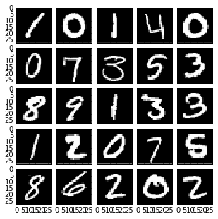
Each row can be reconstructed into a 28x28 array. Here are some examples of random reshaped rows:

The information

Eventually we'll want to train a classifier with these digits, and will want to figure out which features (pixels) are important, and which ones aren't. There are plenty of ways to do that automatically, but it's also straightforward to poke at the data a bit and figure it out ahead of time. First, let's make sure we have the same number of examples for each numeral. The raw data array actually has a prepended "label" column that I didn't mention above, which is just the numeral index, 0-9. We can use this to make a histogram:

where we see that there are about 4000 examples of each numeral.

Next, let's look at what range of intensities we have. Making a histogram of all of the intensities for the entire data set, we see the following:

where it's clear that the data mostly consist of black and white pixels, and not much in between. This gives us a hint that we could binarize the data set without losing much information. It also might mean that there's been some pre-processing done on the data set.

How much does each numeral change throughout the data set? We can get some intuition by grouping examples of each numeral and then plotting their means and variances.

Means of each numeral

Variances of each numeral

These two plots contain more or less the same information - that the variance is concentrated near the edges of each numeral, and there isn't too much variance within each numeral, i.e. there's nothing crazy going on here. Compare this to the average and variance taken over all of the numbers.

We expect variance to correlate well to information, so these images show that most of the information is clustered in a blob near the center, which isn't too surprising. We could probably throw away a bunch of the outer pixels without too much trouble. Let's quantify that.

Suppose we order these pixels by variance (descending) and plot the cumulative variance by pixel. That is, show how adding the next largest variance increases the total variance. That gives us an idea of how many pixels we need to capture most of the variance, which we can expect to be related to information content.

The green line is set at 90% of the total variance, which intersects the cumulative variance at about 290 pixels. So through this exercise we've learned that we can throw away almost 2/3 of the pixels and still capture about 90% of the information, which will be useful when we start training a classfier.