I've been looking recently at the MNIST data set, which contains thousands of hand-written digits like this:
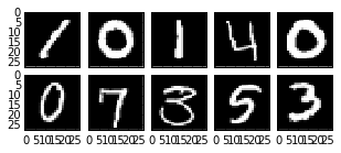 |
| Example hand-written numerals from the MNIST data set |
In part 1 of this series, I looked at the data set and did some preliminary analysis, concluding that:
- There's not much variance within each digit label, i.e. all 5's look pretty much the same.
- Most inter-numeral variance occurs near the center of the field, implying that we can probably throw away the pixels near the edge.
Rather than jumping right into optimizing a classifier in part 2, I'd like to build a validation pipeline. Any time we do machine learning, we want to try to quantify how well our regression or classification should perform on future data. To do otherwise is to leave ourselves prone to errors like overfitting. Validation in this case will apply the classifier to a new set of digits, and then compare the predicted labels to the actual labels.
The Methodology
Here is a pretty concise description of the usual validation methodology. Basically, we break the data into three chunks before we start: a training set, validation set, and test set. Every time we train a classifier we use the training set, and then evaluate its performance using on the validation set. We do that iteratively while tuning metaparameters until we're happy with the classifier, and then test it on the test set. Since we use the validation set to tune the classifier, it sort of "contaminates" it with information, which is why we need the pristine test set. It gives us a better indicator of how the classifier will perform with new data.The pipeline
What do we want our validation suite to look like? It might include:- Standard goodness-of-fit scores, like precision, accuracy, or F1 scores.
- Confusion matrices, which illustrate what numerals are likely to be assigned which incorrect labels (e.g. "6" is likely to be labeled "8")
- Classifier-specific performance plots to evaluate hyperparameters, like regularization constants. These show the training and test error vs. each hyperparameter.
Example: logistic classification
It will be helpful to have a classifier to train in order to build the validation pipeline, so let's choose a simple one. A logistic classifier is a logistic regression in which we apply a threshold to the probability density function to classify a data point. Besides being simple, it's also not going to work very well. For illustrative purposes, that's perfect. I'd like to look at how the performance changes with the hyperparameters, which won't be possible if the performance is close to perfect.
I'm using IPython Notebook again, and I've uploaded the notebook to GitHub so you can follow along, but I'll also paste in some code in case you just want to copy it (please copy away!).
We're just going to use the logistic regression functionality from SciKit-Learn. First I import the data and split it into three groups. 70% goes to training, and 15% each to validation and test sets.
Here I implement a logistic regression with a linear kernel from SciKit-learn. To do some basic validation, I'll just choose a regularization parameter (C in this case) and train the classifier.
Then we can create a validation report, which includes precision, recall, and F1 score for each numeral.
It's a bit easier for me to parse things in visual format, so I also made an image out of the confusion matrix. I set the diagonal elements (which were classified correctly) to zero to increase the contrast.

Whiter squares indicate more misclassifications. We see that the most frequent mistake is that "4" tends to get classified as "9", but we also tend to over-assign the numeral "8" to inputs of "1", "2", and "5". Interestingly, this is not a symmetric matrix, so for example we tend to assign the right label to "8" as an input.

In this plot, larger values mean that the classifier is doing a better job, with 1.00 implying perfect classification. On the horizontal axis, larger values mean less regularization. The red squares show that as we weaken the regularization, the classifier does a better job with the training data. But the performance on the validation data improves for a bit, and then slowly degrades. So for very little regularization, we have overfitting. From a probabilistic point of view, the classifier is no longer representative of the ensemble from which we draw the data.
The validation score peaks around $C\approx 10^{-2.5}$, so even though I've trained on a small subset of the data, I would use this value moving forward.
Now let's make the same graph using $l1$ regularzation.
 The same trends are present here, but the exact value of the optimum is different - around $C\approx 10^{-5.5}$. As a nice illustration, we can run the classifier with this value and see which pixels it elminates. To do that, we retrieve the coefficients from the classifier, of which we get one per pixel per numeral. Keeping only those pixels whose coefficients are $>0$ for at least one of the numerals generates this map:

 and we see that our hunch was correct. The classifier preferentially kept the high-variance pixels.
Now that we have this pipeline, we should be able to use it for other classifiers. The exact analysis will likely change, but at least we'll have a basis for comparison.
I'm using IPython Notebook again, and I've uploaded the notebook to GitHub so you can follow along, but I'll also paste in some code in case you just want to copy it (please copy away!).
We're just going to use the logistic regression functionality from SciKit-Learn. First I import the data and split it into three groups. 70% goes to training, and 15% each to validation and test sets.
 |
| Partitioning the data into training, validation, and test sets. |
Here I implement a logistic regression with a linear kernel from SciKit-learn. To do some basic validation, I'll just choose a regularization parameter (C in this case) and train the classifier.
Then we can create a validation report, which includes precision, recall, and F1 score for each numeral.
It's a bit easier for me to parse things in visual format, so I also made an image out of the confusion matrix. I set the diagonal elements (which were classified correctly) to zero to increase the contrast.
Whiter squares indicate more misclassifications. We see that the most frequent mistake is that "4" tends to get classified as "9", but we also tend to over-assign the numeral "8" to inputs of "1", "2", and "5". Interestingly, this is not a symmetric matrix, so for example we tend to assign the right label to "8" as an input.
Hyperparameters
If we stick with models that are linear in each pixel value, the only hyperparameter we need to choose for logistic regression is the regularization constant, which controls to what degree we weight the input pixels. The two common regularization choices I'll consider are are $l2$ (ridge regression or Tikhonov regularization), and $l1$ (lasso). The former tends to result in a "smooth" weighting, where we put similar weights on everything, but the total overall weight is small. The latter results in "sparse" weighting, where we eliminate many of the inputs as being noninformative.
If we regularize too little, we'll find that while we have low fit error on the training set, we have large errors on the validation set, which is called overfitting. If we regularize too much, we'll find that we're ignoring important information from the input, resulting in large errors for th training and validation sets. This is called underfitting, and the error is called bias.
It can be useful to plot the training and validation error as a function of the regularization constants to see where the regularization performs best. And since we have a pretty large data set, I'll take only a small fraction of the training set. This will make the training go faster, and will just give us an idea of the parameters we should use in the classifier. Let's look at l2 regularization first.
In this plot, larger values mean that the classifier is doing a better job, with 1.00 implying perfect classification. On the horizontal axis, larger values mean less regularization. The red squares show that as we weaken the regularization, the classifier does a better job with the training data. But the performance on the validation data improves for a bit, and then slowly degrades. So for very little regularization, we have overfitting. From a probabilistic point of view, the classifier is no longer representative of the ensemble from which we draw the data.
The validation score peaks around $C\approx 10^{-2.5}$, so even though I've trained on a small subset of the data, I would use this value moving forward.
Now let's make the same graph using $l1$ regularzation.
So to recap, white pixels are those the classifier decides to keep if we tell it to get rid of the least informative ones. Compare this to our map of the variance of each pixel:
Now that we have this pipeline, we should be able to use it for other classifiers. The exact analysis will likely change, but at least we'll have a basis for comparison.
No comments:
Post a Comment